Alex-Monahan.github.io
Project maintained by Alex-Monahan Hosted on GitHub Pages — Theme by mattgraham
Python and SQL: Better Together
Python and SQL are complementary - we should focus on how best to integrate them rather than try to replace them!
By Alex Monahan
2021-08-15 (Yes, this is the one date format to rule them all)
LinkedIn
Twitter @__alexmonahan__
The views I express are my own and not my employer’s.
Welcome to my first blog post! I welcome any and all feedback over on Twitter - I’d love to learn from all of you!
There has been some spirited debate over SQL on Tech Twitter in the last few weeks. I am a huge fan of open discussions like this, and I consistently learn something when reading multiple viewpoints. It’s my hope to contribute to a friendly and productive dialog with fellow data folks! Let’s focus on a few positives from each perspective.
Here, Jamie Brandon makes some excellent points about SQL’s weaknesses. The points I agree with the most are related to SQL’s incompressibility. The way I encounter this most frequently is that it is difficult to execute queries on a dynamic list of columns purely in SQL. I also wish that it was easier to modularize code into functions in more powerful way, although there are some ways of doing so. Imagine a repository of SQL helper functions you could import! If only it were possible. If it is, please let me know on Twitter!
Pedram Navid responded to those points in an indirect way that I also found to be very impactful and thought provoking. Pedram focused on the organizational impacts of choosing to move away from SQL. I agree with Pedram that SQL is a tremendous data democratization tool and that it is important that SQL folks and other programming language folks work as a team. He also makes the case that SQL is often good enough, and I would go a step further and say there are many cases where SQL is a very expressive way to request and manipulate data! The cases where SQL is most useful are very accessible and can really empower people where data is just a portion of their job. SQL is the easiest to learn superpower as a data person!
Pedram also cites dbt as a powerful way to address some of SQL’s rough edges. I would like to take that line of thinking a step further here: How can we mix and match Python and SQL to get the best of both?
Why use SQL?
Before mixing and matching, why would we want to use SQL in the first place? While I agree with Jamie that it is imperfect, it has many redeeming qualities! Toss any others I’ve forgotten on Twitter!
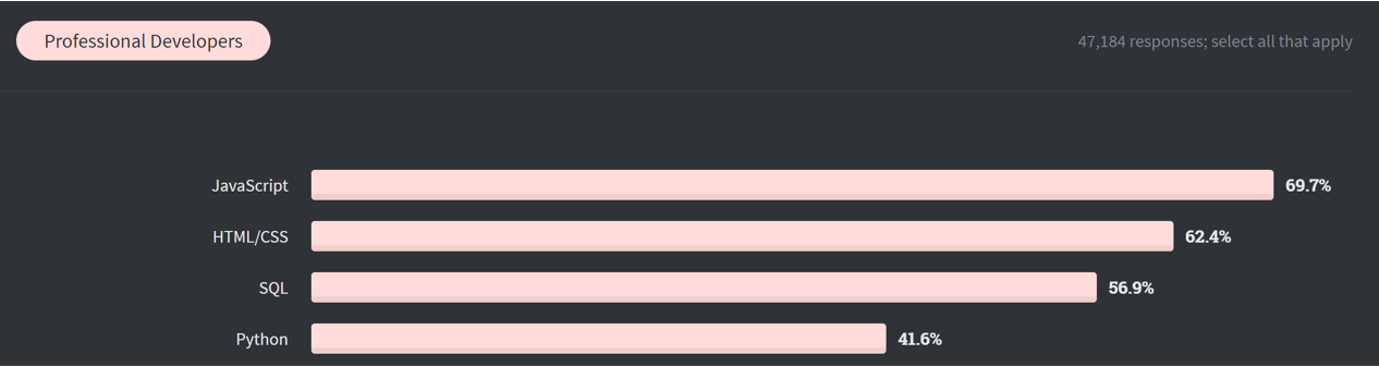
- SQL is very widely used
- It ranks 3rd in the Stack Overflow survey (see above graph!), and it was invented all the way back in 1979!
- Excel and nearly every Business Intelligence tool provide a SQL interface. Plus Python’s standard library includes SQLite, which is in the top 5 most widely deployed pieces of software in existence!
- I also agree with Erik Bernhardsson’s blog post I don’t want to learn your garbage query language. Let’s align on SQL so we only have to learn or develop things once!
- The use of SQL is expanding
- The growth of cloud data warehouses is a huge indication of the power of SQL. Stream processing is adding SQL support, and the SQL language itself continues to grow in power and flexibility.
- SQL is easy to get started with
- While I don’t necessarily have sources to cite here, I have led multiple SQL training courses that can take domain experts from 0 to introductory SQL in 8 hours. While I have not done the same for other languages, I feel like it would be difficult to be productive that quickly!
- However, it’s hard to outgrow the need for SQL
- Even the majority of data scientists use SQL “Sometimes” or more - placing it as the number 2 language in Anaconda’s State of Data Science 2021.
- This also makes SQL great for your career!
- SQL’s declarative nature removes the need to understand database internals
- The deliberate separation between the user’s request and the specific algorithms used by the database is an excellent abstraction layer 99%+ of the time. You can write years of productive SQL queries before learning the difference between a hash join and a sorted merge loop join! And even then, the database will usually choose correctly on your behalf.
- Chances are good you need to use SQL to pull your data initially anyway
- If you already need to know some SQL to access your company’s valuable info, why not maximize your effectiveness with it?
- If you already need to know some SQL to access your company’s valuable info, why not maximize your effectiveness with it?
Tools to use when combining SQL and Python

Asterisks indicate libraries I have not used yet, but that I am excited to try!
- DuckDB
- Think of this as SQLite for analytics! I list the many pros of DuckDB below. It is my favorite way to mix and match SQL and Pandas.
- SQLite
- SQLite is an easy way to process larger than memory data in Python. It comes bundled in the standard library.
- There are a few drawbacks that DuckDB addresses:
- Slow performance for analytics (row-based instead of columnar like Pandas and DuckDB)
- Requires data to be inserted into SQLite before executing a query on it
- Overly flexible data types (This is debatable, but it makes it harder to interact with Pandas in my experience)
- SQLAlchemy
- SQLAlchemy can connect to tons of different databases. It’s a huge advantage for the Python ecosystem.
- When used in combination with pandas.read_sql, SQLAlchemy can pull from a SQL DB and load a Pandas DataFrame.
- SQLAlchemy is traditionally known for its ORM (Object Relational Mapper) capabilities which allow you to avoid SQL. However, it also has powerful features for SQL fans like safe parameter escaping
- There are many other tools for querying SQL DB’s
- ipython-sql
- Convert a Jupyter cell into a SQL language cell! This enables syntax highlighting for SQL in Jupyter.
- I find this much nicer than working with SQL in multi-line strings, and you get syntax highlighting without having separate SQL files.
- This builds on top of SQLAlchemy
- See an example below!
- PostgreSQL’s PL/Python*
- You can write functions and procedures on Postgres using Python!
- I think this addresses some of the concerns highlighted by Jamie Brandon, but as popular as Postgres is, it’s not a standard feature of all DBs
- This is a more DB-centric approach. I’ve found DB stored procedures to be more challenging to use with version control, but they certainly have value
- Dask-sql*
- Process SQL statements on a Dask cluster (on your local machine or 1000’s of servers!)
- The first bullet in the readme advertises easy Python and SQL interoperability, which sounds great!
- This comes with some extra complexity over DuckDB - you’ll need Java for the Apache Calcite query parser and a few lines of code to set up a Dask cluster.
- I’d like to benchmark this a bit to see how well it performs in my single machine use case
- dbt*
- dbt is a way to build SQL pipelines and execute jinja-templated SQL
- The templating seems like a powerful way to avoid some of SQL’s pain points like a rigid set of columns and requiring columns be specified in the SELECT and GROUP BY clauses.
- dbt also works well with version control systems
- I am very excited to try it out, but I am not a cloud data warehouse user so I am slightly outside their target audience
- There are adapters for both DuckDB and Clickhouse (A fast, massively popular open source columnar data warehouse) so this should perform well. These are both community maintained, so I’ll just need to test them out a bit!
I plan to explore more of these in upcoming posts!
DuckDB - One powerful way to mix Python and SQL
![]()
DuckDB is best summarized as the SQLite of analytics. In under 10ms, you can spin up your own in-process database that is 20x faster than SQLite, and in most cases faster than Pandas!
Besides the speed, why do I love DuckDB?
- It works seamlessly with Pandas
- You can query a DataFrame without needing to insert it into the DB, and you can return results as DF’s as well. This is both simple and very fast since it is in the same process as Python.
- Setup is easy
- Just pip install duckdb and you’re all set.
- DuckDB supports almost all of PostgreSQL’s syntax, but also smooths rough edges
- When I first tested out DuckDB, it could handle everything I threw at it: Recursive CTE’s, Window functions, arbitrary subqueries, and more. Even lateral joins are supported! Since then, it has only improved by adding Regex, statistical functions, and more!
- As an example of smoothing rough edges, Postgres is notoriously picky about capitalization, but DuckDB is not case sensitive. While most function names come from Postgres, many equivalent function names from other DB’s can also be used.
-
MIT licensed
- Parquet, csv, and Apache Arrow structures can also be queried by DuckDB
- Interoperability with Arrow and Parquet in particular expand the ecosystem that DuckDB can interact with.
- DuckDB continues to dramatically improve, and the developers are fantastic!
- Truthfully, this should be item 0! I’ve had multiple (sometimes tricky) bugs be squashed in a matter of days, and many of my feature requests have been added. The entire team is excellent!
- Persistence comes for free, but is optional! This allows DuckDB to work on larger-than-memory data.
- If you are building a data pipeline, it can be super useful to see all of the intermediate steps. Plus, I believe that DuckDB databases are going to become a key multi-table data storage structure, just as SQLite is today. The developers are in the midst of adding some powerful compression to DuckDB’s storage engine, so I see significant potential here.
- Did I mention it’s fast?
- DuckDB is multi-threaded, so you can utilize all your CPU cores without any work on your end - no need to partition your data or anything!
- DuckDB has a Relational API that is targeting Pandas compatibility
- While I am admittedly a SQL fan, having a relational API can be very helpful to add in some of the dynamism and flexibility of Pandas.
- While I am admittedly a SQL fan, having a relational API can be very helpful to add in some of the dynamism and flexibility of Pandas.
An example workflow with DuckDB
#I use Anaconda, so Pandas, and SQLAlchemy are already installed. Otherwise pip install those to start with
# !pip install pandas
# !pip install sqlalchemy

!pip install duckdb==0.2.8

#This is a SQLalchemy driver for DuckDB. It powers the ipython-sql library below
#Thank you to the core developer of duckdb_engine, Elliana May!
#She rapidly added a feature and squashed a bug so that it works better with ipython-sql!
!pip install duckdb_engine==0.1.8rc4

#This allows for the %%sql magic in Jupyter to build SQL language cells!
!pip install ipython-sql
import duckdb
import pandas as pd
import sqlalchemy
#no need to import duckdb_engine - SQLAlchemy will auto-detect the driver needed based on your connection string!
Let’s play with a moderately sized dataset: a 1.6 GB csv
This analysis is inspired by this DuckDB intro article by Uwe Korn and can be downloaded here. Note that DuckDB can handle much larger datasets - this is only an example!
First we load the ipython-sql extension and default our output to be in Pandas DF format. We will also simplify what is printed after each SQL statement.
Next, we connect to an in-memory DuckDB and set it to use all our available CPU horsepower!
%load_ext sql
%config SqlMagic.autopandas=True
%config SqlMagic.feedback = False
%config SqlMagic.displaycon = False

%sql duckdb:///:memory:
%sql pragma threads=16
Check out this super clean syntax for directly querying a CSV file! As a note, we could have also used pandas.read_csv and then queried the resulting DataFrame. DuckDB’s csv reader allows us to skip a step!
%%sql
create table taxis as
SELECT * FROM 'yellow_tripdata_2016-01.csv';
| Count | |
|---|---|
| 0 | 10906858 |
Our csv import took 15 seconds: 40% faster than the 25 seconds Pandas required!
(the csv was loaded into RAM prior to timing so it may take an extra few seconds in both cases if you weren’t already working with that file)
Now let’s take a quick sample of our dataset and load it into a Pandas DF.
%%sql
SELECT
    *
FROM taxis
USING SAMPLE 5
| VendorID | tpep_pickup_datetime | tpep_dropoff_datetime | passenger_count | trip_distance | pickup_longitude | pickup_latitude | RatecodeID | store_and_fwd_flag | dropoff_longitude | dropoff_latitude | payment_type | fare_amount | extra | mta_tax | tip_amount | tolls_amount | improvement_surcharge | total_amount | |
|---|---|---|---|---|---|---|---|---|---|---|---|---|---|---|---|---|---|---|---|
| 0 | 2 | 2016-01-29 17:59:21 | 2016-01-29 18:17:50 | 2 | 2.36 | -73.990707 | 40.756535 | 1 | N | -73.991417 | 40.735207 | 1 | 13.0 | 1.0 | 0.5 | 2.96 | 0.0 | 0.3 | 17.76 |
| 1 | 2 | 2016-01-06 20:46:10 | 2016-01-06 20:49:45 | 1 | 0.66 | -73.983322 | 40.750511 | 1 | N | -73.994217 | 40.755001 | 1 | 4.5 | 0.5 | 0.5 | 1.00 | 0.0 | 0.3 | 6.80 |
| 2 | 1 | 2016-01-09 13:23:12 | 2016-01-09 13:29:04 | 1 | 0.50 | -73.994179 | 40.751106 | 1 | N | -73.985992 | 40.750496 | 2 | 5.5 | 0.0 | 0.5 | 0.00 | 0.0 | 0.3 | 6.30 |
| 3 | 2 | 2016-01-28 09:57:02 | 2016-01-28 10:04:10 | 2 | 3.22 | -73.989326 | 40.742462 | 1 | N | -74.002136 | 40.709290 | 1 | 11.0 | 0.0 | 0.5 | 1.50 | 0.0 | 0.3 | 13.30 |
| 4 | 2 | 2016-01-18 20:45:15 | 2016-01-18 21:06:36 | 1 | 13.80 | -74.012917 | 40.706169 | 1 | N | -73.939781 | 40.852749 | 1 | 37.5 | 0.5 | 0.5 | 3.80 | 0.0 | 0.3 | 42.60 |
As you can see below, DuckDB did a great job auto-detecting our column types. One more traditional DB hassle eliminated!
%sql describe taxis
| Field | Type | Null | Key | Default | Extra | |
|---|---|---|---|---|---|---|
| 0 | VendorID | INTEGER | YES | None | None | None |
| 1 | tpep_pickup_datetime | TIMESTAMP | YES | None | None | None |
| 2 | tpep_dropoff_datetime | TIMESTAMP | YES | None | None | None |
| 3 | passenger_count | INTEGER | YES | None | None | None |
| 4 | trip_distance | DOUBLE | YES | None | None | None |
| 5 | pickup_longitude | DOUBLE | YES | None | None | None |
| 6 | pickup_latitude | DOUBLE | YES | None | None | None |
| 7 | RatecodeID | INTEGER | YES | None | None | None |
| 8 | store_and_fwd_flag | VARCHAR | YES | None | None | None |
| 9 | dropoff_longitude | DOUBLE | YES | None | None | None |
| 10 | dropoff_latitude | DOUBLE | YES | None | None | None |
| 11 | payment_type | INTEGER | YES | None | None | None |
| 12 | fare_amount | DOUBLE | YES | None | None | None |
| 13 | extra | DOUBLE | YES | None | None | None |
| 14 | mta_tax | DOUBLE | YES | None | None | None |
| 15 | tip_amount | DOUBLE | YES | None | None | None |
| 16 | tolls_amount | DOUBLE | YES | None | None | None |
| 17 | improvement_surcharge | DOUBLE | YES | None | None | None |
| 18 | total_amount | DOUBLE | YES | None | None | None |
Now let’s do some analysis!
First, let’s see how we can pass in a parameter through ipython-sql to better understand how VendorId 1 is behaving. Just for fun, we are going to pass in the entire WHERE clause. Why? It shows that you can build up dynamic SQL statements using Python! It’s not quite as easy to use as a templating language, but just as flexible.
my_where_clause = """
    WHERE
        vendorid = 1
"""
%%sql
SELECT
    vendorid
    ,passenger_count
    ,count(*) as count
    ,avg(fare_amount/total_amount) as average_fare_percentage
    ,avg(trip_distance) as average_distance
FROM taxis
{my_where_clause}
GROUP BY
    vendorid
    ,passenger_count
| VendorID | passenger_count | count | average_fare_percentage | average_distance | |
|---|---|---|---|---|---|
| 0 | 1 | 0 | 303 | 0.480146 | 3.217492 |
| 1 | 1 | 1 | 4129971 | 0.787743 | 6.362515 |
| 2 | 1 | 2 | 689305 | 0.796871 | 5.674639 |
| 3 | 1 | 3 | 164253 | 0.804641 | 3.126398 |
| 4 | 1 | 4 | 83817 | 0.819123 | 32.439788 |
| 5 | 1 | 5 | 2360 | 0.806479 | 3.923771 |
| 6 | 1 | 6 | 1407 | 0.788484 | 3.875124 |
| 7 | 1 | 7 | 3 | 0.755823 | 4.800000 |
| 8 | 1 | 9 | 10 | 0.785628 | 3.710000 |
Next we’ll aggregate our data in DuckDB (which is exceptionally fast for Group By queries), and then pivot the result with Pandas. Pandas is a great fit for pivoting because the column names are not known ahead of time, which would require writing some dynamic SQL. However, DuckDB has a pivot_table function on their roadmap for their Python Relational (read, DataFrame-like) API! This will allow us to pivot larger than memory data and use multiple CPU cores for that pivoting operation.
Note: The more complex the query, the better DuckDB performs relative to Pandas! This is because it can do more work in less passes through the dataset, and because it is using multiple CPU cores.
%%sql aggregated_df <<
SELECT
    --Aggregate up to a weekly level. lpad makes sure week numbers always have 2 digits (Ex: '02' instead of '2')
    date_part('year',tpep_pickup_datetime) ||
        lpad(cast(date_part('week',tpep_pickup_datetime) as varchar),2,'0') as yyyyww
    ,passenger_count
    ,count(*) as count
    ,min(total_amount) as min_amount
    ,quantile_cont(total_amount,0.1) as _10th_percentile
    ,quantile_cont(total_amount,0.25) as _25th_percentile
    ,quantile_cont(total_amount,0.5) as _50th_percentile
    ,avg(total_amount) as avg_amount
    ,quantile_cont(total_amount,0.75) as _75th_percentile
    ,quantile_cont(total_amount,0.9) as _90th_percentile
    ,max(total_amount) as max_amount
    ,stddev_pop(total_amount) as std_amount
FROM taxis
GROUP BY
    date_part('year',tpep_pickup_datetime) ||
        lpad(cast(date_part('week',tpep_pickup_datetime) as varchar),2,'0')
    ,passenger_count
ORDER BY
    yyyyww
    ,passenger_count
Returning data to local variable aggregated_df
aggregated_df
| yyyyww | passenger_count | count | min_amount | _10th_percentile | _25th_percentile | _50th_percentile | avg_amount | _75th_percentile | _90th_percentile | max_amount | std_amount | |
|---|---|---|---|---|---|---|---|---|---|---|---|---|
| 0 | 201601 | 0 | 129 | -160.46 | 3.000000e-01 | 4.8000 | 10.560 | 21.901163 | 22.5600 | 70.019999 | 278.30 | 45.119609 |
| 1 | 201601 | 1 | 1814315 | -227.10 | 6.350000e+00 | 8.1800 | 11.160 | 14.909425 | 16.3000 | 26.300000 | 3045.34 | 12.835089 |
| 2 | 201601 | 2 | 361892 | -100.80 | 6.800000e+00 | 8.3000 | 11.620 | 15.835135 | 17.1600 | 29.300000 | 1297.75 | 14.113061 |
| 3 | 201601 | 3 | 100336 | -80.80 | 6.800000e+00 | 8.3000 | 11.300 | 15.394737 | 16.6200 | 27.300000 | 1297.75 | 14.566035 |
| 4 | 201601 | 4 | 47683 | -120.30 | 6.800000e+00 | 8.3000 | 11.300 | 15.561985 | 16.8000 | 28.300000 | 889.30 | 13.701526 |
| 5 | 201601 | 5 | 138636 | -52.80 | 6.360000e+00 | 8.3000 | 11.300 | 15.263942 | 16.6200 | 27.960000 | 303.84 | 12.353158 |
| 6 | 201601 | 6 | 85993 | -52.80 | 6.360000e+00 | 8.1900 | 11.160 | 14.889752 | 16.3000 | 26.300000 | 170.50 | 11.906014 |
| 7 | 201601 | 7 | 6 | 70.80 | 7.330000e+01 | 76.3675 | 83.685 | 82.648333 | 90.5450 | 90.960000 | 90.96 | 8.069036 |
| 8 | 201601 | 8 | 4 | 8.30 | 8.690000e+00 | 9.2750 | 9.805 | 36.630000 | 37.1600 | 86.029992 | 118.61 | 47.335385 |
| 9 | 201601 | 9 | 1 | 11.80 | 1.180000e+01 | 11.8000 | 11.800 | 11.800000 | 11.8000 | 11.800000 | 11.80 | 0.000000 |
| 10 | 201602 | 0 | 137 | -10.10 | 3.000000e-01 | 6.3500 | 13.390 | 24.970073 | 35.3000 | 70.513999 | 148.01 | 30.159674 |
| 11 | 201602 | 1 | 1911279 | -150.30 | 6.360000e+00 | 8.3000 | 11.300 | 15.160333 | 16.5500 | 27.300000 | 1297.75 | 13.008159 |
| 12 | 201602 | 2 | 383117 | -200.80 | 6.800000e+00 | 8.3000 | 11.750 | 15.868765 | 17.1600 | 29.300000 | 1154.84 | 14.086363 |
| 13 | 201602 | 3 | 107589 | -52.80 | 6.800000e+00 | 8.3000 | 11.300 | 15.317193 | 16.8000 | 27.300000 | 472.94 | 12.881864 |
| 14 | 201602 | 4 | 50919 | -958.40 | 6.800000e+00 | 8.3000 | 11.300 | 15.412864 | 16.8000 | 27.950000 | 958.40 | 14.208739 |
| 15 | 201602 | 5 | 147897 | -54.80 | 6.360000e+00 | 8.3000 | 11.300 | 15.380488 | 16.8000 | 28.340000 | 240.80 | 12.517914 |
| 16 | 201602 | 6 | 91826 | -52.80 | 6.360000e+00 | 8.3000 | 11.300 | 15.058432 | 16.5600 | 27.300000 | 200.00 | 12.108098 |
| 17 | 201602 | 7 | 2 | 8.10 | 8.365000e+00 | 8.7625 | 9.425 | 9.425000 | 10.0875 | 10.485000 | 10.75 | 1.325000 |
| 18 | 201602 | 8 | 6 | 5.80 | 7.050000e+00 | 8.7250 | 10.100 | 36.156667 | 63.1500 | 91.319997 | 101.84 | 39.502676 |
| 19 | 201602 | 9 | 6 | -9.60 | 1.430511e-07 | 9.7250 | 11.360 | 36.283333 | 57.2825 | 97.489994 | 122.81 | 46.255662 |
| 20 | 201603 | 0 | 110 | 0.00 | 3.000000e-01 | 0.9275 | 11.460 | 30.601818 | 53.1750 | 90.259985 | 282.30 | 42.165426 |
| 21 | 201603 | 1 | 1526446 | -200.80 | 6.800000e+00 | 8.5000 | 11.760 | 15.951602 | 17.3000 | 29.000000 | 8008.80 | 16.090206 |
| 22 | 201603 | 2 | 281137 | -75.30 | 6.800000e+00 | 8.7600 | 12.250 | 16.938134 | 18.3000 | 32.800000 | 725.30 | 15.298718 |
| 23 | 201603 | 3 | 76414 | -75.84 | 6.800000e+00 | 8.7600 | 11.800 | 16.356485 | 17.7600 | 29.800000 | 1137.85 | 15.731051 |
| 24 | 201603 | 4 | 35166 | -73.80 | 6.800000e+00 | 8.7600 | 11.800 | 16.261706 | 17.7600 | 30.800000 | 459.79 | 14.083521 |
| 25 | 201603 | 5 | 117191 | -52.80 | 6.800000e+00 | 8.7600 | 11.800 | 16.123766 | 17.7600 | 30.300000 | 271.30 | 13.284821 |
| 26 | 201603 | 6 | 70617 | -52.80 | 6.800000e+00 | 8.5000 | 11.760 | 15.869602 | 17.3000 | 29.300000 | 326.84 | 12.932498 |
| 27 | 201603 | 7 | 5 | 7.60 | 7.788000e+00 | 8.0700 | 8.100 | 29.332000 | 46.5900 | 64.415997 | 76.30 | 27.853121 |
| 28 | 201603 | 8 | 5 | 8.80 | 9.120000e+00 | 9.6000 | 80.800 | 58.760000 | 95.3000 | 97.700000 | 99.30 | 40.931973 |
| 29 | 201603 | 9 | 3 | 10.10 | 1.164000e+01 | 13.9500 | 17.800 | 42.233333 | 58.3000 | 82.599996 | 98.80 | 40.122008 |
| 30 | 201604 | 0 | 80 | -0.80 | 3.000000e-01 | 1.1750 | 17.945 | 33.452375 | 62.7625 | 80.300000 | 132.80 | 33.498167 |
| 31 | 201604 | 1 | 1622846 | -440.34 | 6.800000e+00 | 8.7600 | 12.300 | 16.211807 | 18.3000 | 29.160000 | 111271.65 | 88.344714 |
| 32 | 201604 | 2 | 323779 | -234.80 | 6.950000e+00 | 8.8000 | 12.360 | 16.718532 | 18.8000 | 30.950000 | 795.84 | 13.931410 |
| 33 | 201604 | 3 | 89060 | -52.80 | 6.850000e+00 | 8.8000 | 12.300 | 16.218767 | 18.3000 | 29.160000 | 724.82 | 13.392155 |
| 34 | 201604 | 4 | 41461 | -52.80 | 6.890000e+00 | 8.8000 | 12.300 | 16.079813 | 18.3000 | 28.800000 | 249.35 | 12.625694 |
| 35 | 201604 | 5 | 126134 | -52.80 | 6.800000e+00 | 8.8000 | 12.300 | 16.341509 | 18.3600 | 30.290000 | 259.80 | 12.791541 |
| 36 | 201604 | 6 | 77699 | -52.80 | 6.800000e+00 | 8.8000 | 12.300 | 16.129398 | 18.3000 | 29.750000 | 177.46 | 12.564739 |
| 37 | 201604 | 7 | 5 | 8.10 | 9.460000e+00 | 11.5000 | 18.170 | 37.074000 | 70.0000 | 74.559999 | 77.60 | 30.256773 |
| 38 | 201604 | 8 | 5 | 10.38 | 1.046800e+01 | 10.6000 | 80.800 | 60.596000 | 98.8400 | 100.952000 | 102.36 | 41.560278 |
| 39 | 201604 | 9 | 5 | 10.80 | 4.360000e+01 | 92.8000 | 97.800 | 82.100000 | 100.3000 | 105.399999 | 108.80 | 36.024436 |
| 40 | 201653 | 0 | 64 | -7.80 | 3.000000e-01 | 1.1425 | 11.775 | 24.791719 | 34.7250 | 73.869993 | 107.30 | 29.413893 |
| 41 | 201653 | 1 | 852098 | -300.80 | 6.300000e+00 | 7.8000 | 10.800 | 15.229454 | 16.5600 | 29.120000 | 1003.38 | 13.651999 |
| 42 | 201653 | 2 | 212052 | -258.20 | 6.360000e+00 | 8.3000 | 11.300 | 16.580428 | 17.7600 | 34.240000 | 1004.94 | 15.547422 |
| 43 | 201653 | 3 | 63032 | -75.30 | 6.360000e+00 | 8.3000 | 11.300 | 16.141369 | 17.3000 | 31.340000 | 998.30 | 15.105769 |
| 44 | 201653 | 4 | 35412 | -100.30 | 6.800000e+00 | 8.3000 | 11.400 | 16.463965 | 17.3000 | 32.195966 | 656.15 | 15.957624 |
| 45 | 201653 | 5 | 71221 | -21.30 | 6.300000e+00 | 8.1600 | 11.160 | 15.816108 | 17.1600 | 32.300000 | 469.30 | 13.725301 |
| 46 | 201653 | 6 | 43020 | -52.80 | 6.300000e+00 | 7.8800 | 11.000 | 15.358045 | 16.6400 | 30.300000 | 148.34 | 13.060431 |
| 47 | 201653 | 7 | 4 | 8.20 | 8.665000e+00 | 9.3625 | 40.025 | 45.147500 | 75.8100 | 85.727998 | 92.34 | 37.006354 |
| 48 | 201653 | 8 | 6 | 9.60 | 4.495000e+01 | 80.4250 | 80.800 | 77.088333 | 84.5800 | 105.514995 | 125.19 | 34.114769 |
| 49 | 201653 | 9 | 8 | 5.80 | 7.025000e+00 | 7.7375 | 8.400 | 10.331250 | 12.0125 | 15.004999 | 20.15 | 4.291994 |
pivoted_df = pd.pivot_table(aggregated_df,
               values=['_50th_percentile'],
               index=['yyyyww'],
               columns=['passenger_count'],
               aggfunc='max'
            )
pivoted_df
| _50th_percentile | ||||||||||
|---|---|---|---|---|---|---|---|---|---|---|
| passenger_count | 0 | 1 | 2 | 3 | 4 | 5 | 6 | 7 | 8 | 9 |
| yyyyww | ||||||||||
| 201601 | 10.560 | 11.16 | 11.62 | 11.3 | 11.3 | 11.30 | 11.16 | 83.685 | 9.805 | 11.80 |
| 201602 | 13.390 | 11.30 | 11.75 | 11.3 | 11.3 | 11.30 | 11.30 | 9.425 | 10.100 | 11.36 |
| 201603 | 11.460 | 11.76 | 12.25 | 11.8 | 11.8 | 11.80 | 11.76 | 8.100 | 80.800 | 17.80 |
| 201604 | 17.945 | 12.30 | 12.36 | 12.3 | 12.3 | 12.30 | 12.30 | 18.170 | 80.800 | 97.80 |
| 201653 | 11.775 | 10.80 | 11.30 | 11.3 | 11.4 | 11.16 | 11.00 | 40.025 | 80.800 | 8.40 |
Let’s summarize what we have accomplished!
To go from Python to SQL, we have used Python to generate SQL dynamically and have embedded our SQL code nicely alongside Python in our Jupyter Notebook programming environment. We also discussed using DuckDB to read a Pandas DF directly. When moving from SQL to Python, DuckDB can quickly and easily convert SQL results back into Pandas DF’s. Now we can mix and match Python and SQL to our heart’s content!
Thank you for reading! Please hop on Twitter and let me know if any of this was helpful or what I can cover next!